I analyze vegetation of the Yatsugatake Mountains using QGIS

• English
• 日本語

The GIS is software (Geographic Information System) handling map space information. It was the thing which I could treat only in a company engaged in specialized duties (expensive) before, but it was in free & open source called QGIS (Quantum GIS) now, and the data which were enormous if I learned a little came to be available freely. I noticed a thing called this just recently, but I finally found a primer of QGIS in a bookstore and bit it a little.

There has been reviewing it of being related of vegetating (having taken several months) with the topography of the Yatsugatake Mountaions which was the study theme 40 years ago in around three days. The data which I used are base map information service of Geographical Survey Institute and 1/2, 5000 vegetation map GIS data of Ministry of the Environment Center for Biological Diversity. In brief, all the map information is computerized now. I know the careful ups and downs of the land by laser air survey and can download all a form and the positions such as a road or the building that I read from an aerial photo. I feel like seeming to be able to really do anything if I get know-how to process such a GIS data. There are vector data expressing a position at a coordinate and raster data to display it for an aspect, and to express, but as the raster data are the same as an image to use with astrophotograph, read it as data if I use matplotlib of Python, and it is easily possible for the statistics processing, too. From vegetation data and altitude data of the 10m mesh such as the top, I graphed relations with altitude and the vegetation to grow.

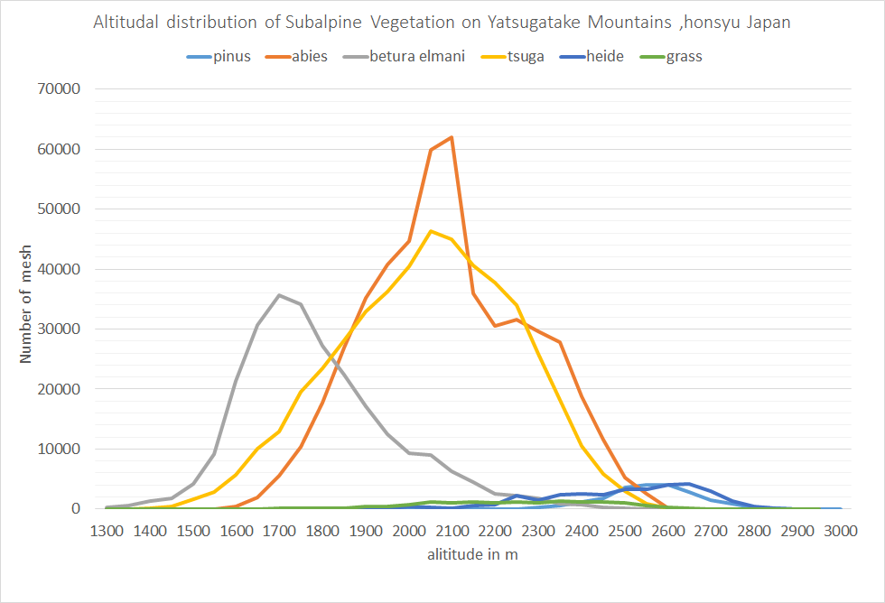
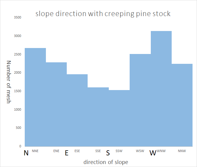
Around 2,500m above sea level of the Japanese central part mountains is called an alpine belt (actually subalpine zone). As for it, a creeping pine and the scenery consisting of fields of flowers spread. I wanted to check what kind of environmental factor it arose in. 40 years ago, I have terminated in the result not to aim at. I can easily show the data except the Yatsugatake, too. I will make one of the pleasure of the old age from now on.

The bottom is a source code of Python which I used for analysis.

"""
Programs for collection of GeoTiff-filetyoe
"""
import csv
import matplotlib
matplotlib.use('Agg') # for printout-file fig-histgram
import matplotlib.pyplot as plt
import numpy as np
from PIL import Image   #PIL;pillow module

xc =[] # list for raw-band data

filename = "tsuga-keisya"   # filename input and output
im = np.array(Image.open(filename +'.tif'))
# print(type(im))   # <class 'numpy.ndarray'>
x = np.ravel(im)   # conversion to list
xl = x.tolist()

for i in xl：   # ignore 0 data  
    if i <= 0:　
        continue
    xc.append(i)

# histgram method by matplotlib
r = plt.hist(xc, bins=16, range=(0,80), normed=False, weights=None,
                       cumulative=False, bottom=None, histtype='bar',
                       align='mid', orientation='vertical', rwidth=1,
                       log=False, color=None, label=None, stacked=False,)
#                       hold=None, data=None, )
# dic = {key: val for key, val in zip(r[1],r[0])}
plt.show()
plt.savefig('histgram.png')
# print(dic)
# output hist_data for csv-file

with open(filename +".csv", "w", newline="") as f:
    w = csv.writer(f,delimiter=",", quotechar='"')

    length = len(r[0])
    for i in range(length):
        w.writerow([r[1][i],r[0][i]])